Conditional Auto Regressive or CAR models are one of the foundational tools for modeling areal level data. In this post we’ll examine some of the different variants of this model, the different strengths and weaknesses each possess and discuss how they can be used in modeling built environment data. This post is largely inspired by the case study by Mitzi et al. with less elaboration on technical details and a novel application to street crime data.
The first two sections focus on the technical details and history in the literature, while the third focuses on how this method can be applied and hints of how it might be used to inform urban policy making.
The CAR model
The CAR family accommodates spatial correlation between spatially adjacent observations through the incorporation of a spatial effect \(b_i\), whose covariance is a function of the spatial adjacency between observations. Specifically, for an areal observation \(y_i\), a linear model with covariate vector \(\mathbf{x}_{i}\) and regression coefficients vector \(\mathbf{\beta}\), would incorporate CAR effects as follows:
\[\begin{equation} \begin{aligned} y_i &= \mathbf{x}^{T}_i\mathbf{\beta} + b_i\\ \mathbf{b} &\sim MVN(\mathbf{0},\Sigma)\\ \Sigma &= \tau D(I-\rho \mathbf{A}), \end{aligned} \tag{1} \end{equation}\]
where \(\Sigma\), the covariance matrix for \(\mathbf{b}\) are a function of scale \(\tau\), difference matrix1 \(D\), adjacency matrix \(\mathbf{A}\)2, and spatial correlation \(\rho\). When \(\rho=1\) the adjacent observations are understood to be completely correlated and when fixing this parameter as such the model is called the Intrinsic Conditional Autoregressive (ICAR) model.
There are various theoretical details that make using CAR and ICAR models problematic. To start, when considering the spatial parameter \(\rho\) unknown, as in the CAR framework, the parameter does not offer an intuitive interpretation; values of \(\rho\) that are not very close to 1 allow for almost no spatial correlation whatsoever and negative spatial correlation usually does not comport with a substantive understanding of the data. As for the ICAR model, by fixing \(\rho=1\), the correlation between observations is understood to be completely driven by spatial association, which can be problematic in situations where there is non-spatial variability, or problems with over-dispersion, as is often in the case with spatial applications modeling counts using, e.g. a Poisson distribution. All of these issues prompted the development of a new approach by Besag, York and Mollie, that strives to take advantage of the inherent intuition behind the ICAR model but also overcome it’s weaknesses. It is to this new framework we now turn our attention, but if the reader is interested in learning more about the details underlying the CAR and ICAR models they should consult chapter 3 of (Banerjee, Carlin, and Gelfand 2003), (Morris et al. 2019) and the latter’s online case study.
The Besag York and Mollie Model
The original paper by Besag York and Mollie (BYM) proposed a model that incorporated the two sources of variability — site specific and spatial variability — previously addressed with one spatial effect term in ICAR models with two types of random effects: a site specific effect independent of spatial correlation, and a spatial effect complete with an ICAR variance structure (Besag, York, and Mollié 1991). The addition of this extra term caused new issues with identifiability and appropriate placement of priors which prompted further work by (Riebler et al. 2016) and others3 to further improve the parameterization introduced by BYM. By introducing a new constraint, shared scale \(\sigma\) and correlation parameter \(\rho\), their model improved identifiability and facilitated a more intuitive placement of priors on the hyper parameters. Denoting the scaled site-specific effect for the \(i\)th location as \(\psi_i\) and the spatial effect as \(\phi_i\) and their original variants as \(\psi_i^{*}\),\(\phi_i^{*}\), the new model specification is as follows:
\[\begin{equation} \begin{aligned} y_i &= \mathbf{x}_{i}\mathbf{\beta} + b_i\\ \mathbf{b}_i &= \psi_i + \phi_i \\ &= \sigma(\sqrt{1-\rho}\psi^{*}_i + \sqrt{\rho}\phi_i^{*}) \\ \psi^{*} &\sim N(0,\mathbf{I})\\ \phi^{*} &\sim N(0,\Sigma^{\star}) \\ \Sigma^{\star} &= D(I-\rho \mathbf{A}). \end{aligned} \tag{2} \end{equation}\]
Note that \(\Sigma^{\star}\) is now scaled and constrained so that \(V[\phi] \approx 1\). With all this machinery in place, the more application driven reader would be well warranted asking if now, we have a model that offers us a better chance of modeling spatially networked data. The short analysis in the following section aspires to show that we do.
BYM Application to Crime and other City Street Events
Turning our attention back to the class of crime data discussed in (Moyer et al. 2019) we look to see how we can improve the methods used in their work to better reflect the level at which more focused policy and community efforts can take effect: city streets.
The reader may recall that the authors used two approaches to estimate the effect of cleaned up vacant lots on the rate of violent shootings not involving police officers in Philadelphia. The first used a kernel density estimate of the shootings, while the second used a simple count within a given buffer — 300 and 600 meters — of the vacant lot. In this section I’d like to propose a method that will simplify the effort of “counting” where crimes occur, and enable a more intuitive modeling framework. Note that I do not (yet) involve the estimation of the effect of vacant lots on the incidence of crime, leaving that topic for a future post.
Mapping Crimes to Streets
The police reports documenting crime by the Philadelphia Police Department, contain a GPS coordinate as the location of the shooting, a single point in space and time, but individuals belonging to neighborhoods similarly understand the crime — and many other similar city events — to have occurred “on a street.” Thus the idea of mapping crimes from the single point location to the closest street by, e.g. euclidean distance4, and using the street as the spatial index where outcomes are measured follows naturally. This idea is illustrated in Figure 1, where shootings regularly occur on a city street or can be understood as occurring on a city street: if an event occurs inside a store whose address corresponds to a street, we would still colloquially understand the crime to have occurred “on the street,” even though the crime did not occur on the asphalt representing the literal physical street.
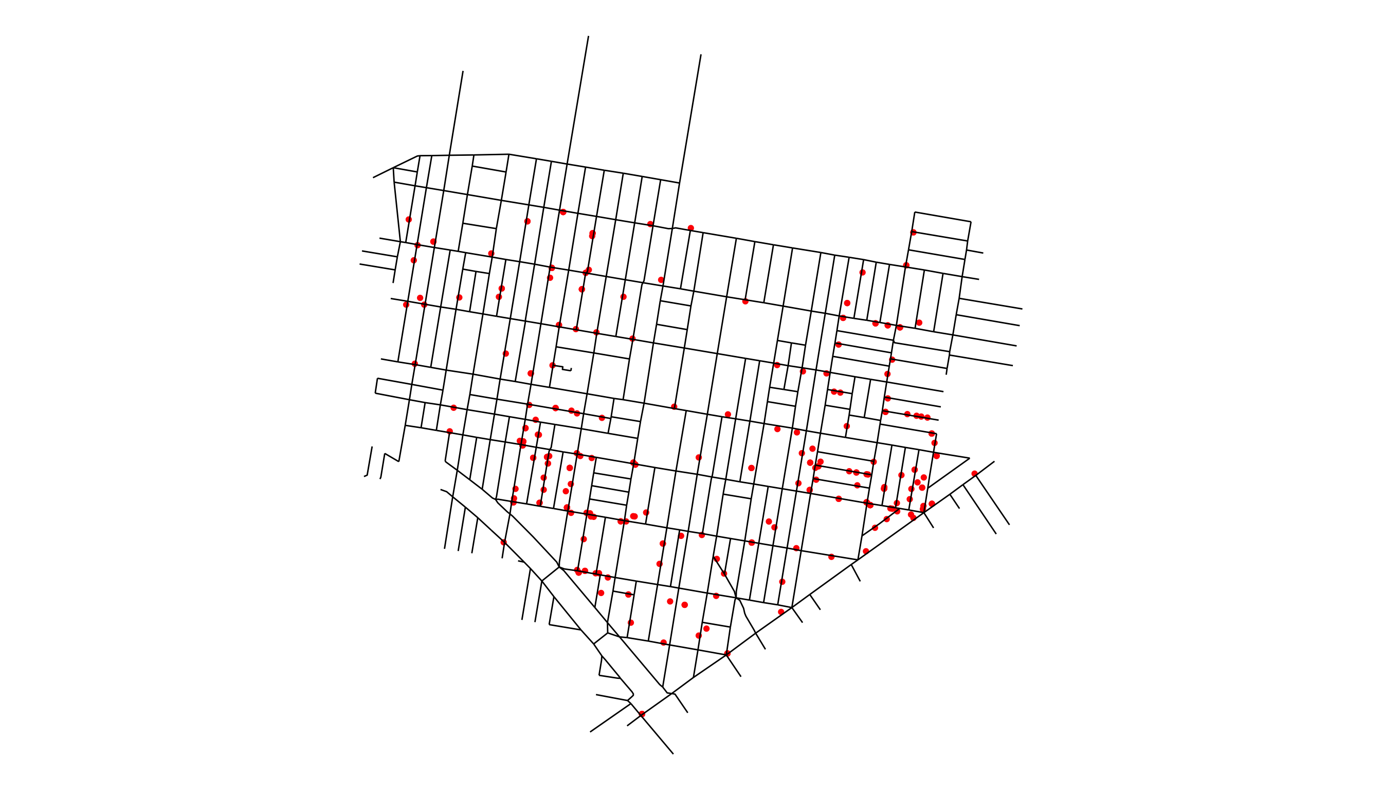
Figure 1: Shootings in the Neighborhood of Upper Kensington during Calendar year 2015. City Street and Crime data are from opendataphilly.org.
Not only does mapping crimes to streets offer an intuitive understanding for modeling city events, such as the shootings studied in (Moyer et al. 2019), the street network also allows us to borrow information across the different streets by street adjacency to model correlation through using, for example, the BYM parameterization of the ICAR prior. The previous modeling framework employed by (Moyer et al. 2019) used a neighborhood specific effect to try and capture this correlation, but by incorporating spatial structure we should be able to improve upon their efforts to more efficiently and accurately estimating the parameters of interest. Figure 2 gives an illustration of how one might visualize the network determined by city streets.
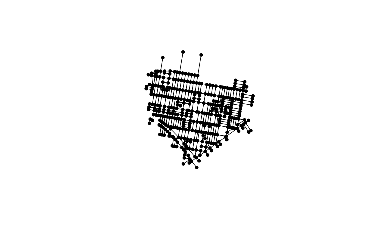
Figure 2: Network visualization of the streets in Upper Kensington. Note that this is not the exact manner in which the network information is used in the Besag York and Mollie model, as the streets are in fact considered to be the nodes of the graph and the street intersections the edges, but the plot is illustrative of the general idea.
Zero Inflated Poisson BYM Model
The use of the BYM model is particularly important in modeling the count of shootings or other events on a particular street as we will need the extra flexibility provided by the random effect \(\psi_i\), described above, to avoid problems with over-dispersion in modeling the counts as distributed from a poisson distribution. City events like shootings, accidents, etc. will typically by zero-inflated, as they do not — typically — occur at such a high frequency across every single street as to receive daily, monthly or possibly even an annual record. Thus, a zero point mass, or zero-inflated model, is critical to accurately modeling the underlying process from which the data are generated. I’ll present, fit and interpret a simple model to briefly illustrate the idea. Let \(Y_{itm}\) be the number of shootings observed at street \(i\), during calendar year \(t\) and month \(m\). Then let \(\pi\) be the probability of an observation being drawn from the zero point mass. Using a similar notation as above for the BYM components, the model is as follows:
\[\begin{equation} \begin{aligned} Y_{itm} \sim \ \pi\delta_{0}(\cdot) + (1-\pi)\text{Pois}(\exp{(\alpha + \text{Year}_{t}\times \beta_t + \gamma_m + b_i)}), \end{aligned} \tag{3} \end{equation}\]
where \(\delta_{0}(\cdot)\) is the dirac delta function at zero, \(\alpha\) is a global intercept, \(\beta_t\) is the difference between year \(t\) and the reference year of 2019,\(\gamma_m\) is a month specific effect, and \(b_i\) is the composite spatial and street specific effect as described in (2).
We can fit this model in the brms package after creating the spatial network and adjacency matrix,A, from functions in the sfnetworks,tidygraph and igraph R packages(van der Meer et al. 2021; Csardi and Nepusz 2006; Pedersen 2020). See the code in the repo to learn more.
fit <- brm(shootings ~  Year + (1|Month) + car(A, gr = OBJECTID,type='bym2'),
           data = mdf,
           data2 = list(A = A),
           family = zero_inflated_poisson(),
           cores = 3,
           chains = 3,
           backend = "cmdstanr",
           threads = threading(2),
           iter = 2E3)
You can see the estimated monthly shooting rates by year in Table 1 which are fairly similar and not of primary interest so I leave them in the details section below. Plotting the composite effects \(b_i\) in Figure 3 we’re able to observe how the rate of shootings varies spatially across the city streets after adjusting for the global and local temporal effects captured by the other parameters, \(\beta_t,\gamma_m\).
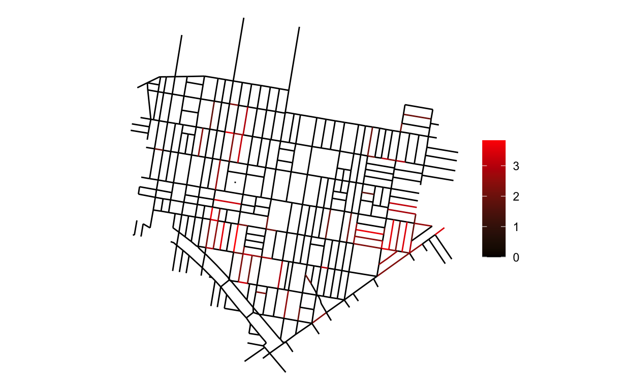
Figure 3: Distribution of median monthly rate ratio deemed credible with 90% probability, as compared to a typical street, of shootings across city streets in Upper Kensington. Non credible effects are shown as 0.
The plot in 3 shows the median log rate ratio of shootings for each street in the Upper Kensington Neighborhood that is determined to be “credibly” non-zero. That is, with 90% probability the model estimates that the effect is greater than 0. We can interpret an example street estimate of 1.97 to indicate that that street has exp(1.97) \(\approx\) 7 times more shootings than a typical street in Kensington (where \(b_i = 0\)), all else equal. Further, you should notice how this plot agrees with Figure 1 which is a nice reinforcement that the model is capturing the data correctly. There is much more that could be learned from this modeling framework. For example, the parameter \(\pi\), could be made street specific, \(\pi_{i}\), so as to identify what features of a street are most likely to be associated with a complete lack of shootings. At this point, hopefully one can start to imagine how this model might be used in the context of urban policy decision making. By identifying those streets that are most at risk, the strength of correlation at the spatial or street specific level, or even just being able to offer a more intuitive interpretation of how policy may affect resident’s lives in a context they can appreciate, there are lots of opportunities. For the sake of brevity, I’ll simply conclude with one final note, a reminder of what this model is and is not saying.
This model is merely descriptive — it is describing the variability of shootings across the Upper Kensington neighborhood streets from 2019-2021 — rather than offering us anything causal as (Moyer et al. 2019)’s work sought to do. This is however, as far as I can tell, the first application of the BYM framework to city street level events5. I hope to show in a future post and possibly a proper paper, how this modeling framework can be combined with other ideas, such as the spatial temporal aggregated predictors I developed alongside my coauthors in (Peterson 2020; Peterson, Hirsch, and Sanchez 2021) to improve the estimate of the vacant lot cleanup effect (Moyer et al. 2019) estimated in their work. Such efforts usually take a long time, but I will post more about that here as soon as any meaningful progress has been made.
| Year | Median (5%,95%) |
|---|---|
| 2019 | 0.02 (0.02, 0.04) |
| 2020 | 0.03 (0.02, 0.07) |
| 2021 | 0.02 (0.01, 0.06) |
where \(D_{i,i}\) is the number of spatially adjacent neighbors for area \(i\) and 0 everywhere else↩︎
where \(A_{i,j} = 1\) indicates area \(i\) and \(j\) are spatially connected and 0 indicates they are not↩︎
(Riebler et al. 2016) contains a nice summary of the work leading up to their model.↩︎
Other distance measures could be used, but at the small distances we are considering the differences should be negligible.↩︎
(Rose et al. 2018) attempted to do something similar using a Gaussian process↩︎