In studying the built environment and furthering our understanding of how to build better urban spaces, we’re often forced to study data that are spatially indexed — that is, the measurement’s spatial location is relevant to the project of interest. In order to handle this class of data we consequently need models that are specifically built to handle that spatial component: a spatial model.
What’s a spatial model and how does it differ from a “non-spatial” model? In this post I’ll give an answer to these questions and more by providing a brief introduction to the three most common classes of spatial data structures and the models most often used with them. While I’ll do my best to build these up from the standard linear model commonly used across many quantitative disciplines, this post is no substitute for the more rigorous presentations offered elsewhere. See (Casella and Berger 2021; Gelman, Hill, and Vehtari 2020) or(Fitzmaurice et al. 2008) for a more thorough introduction to standard regression models, mixed effects models and (Banerjee, Carlin, and Gelfand 2003; Diggle 2006) for a more thorough introduction to spatial models.
The Ordinary Linear Model
One of the very first models introduced in basic statistics curriculum is the “ordinary linear model” shown below with three unknown variables: \(\alpha,\beta\) and \(\sigma^2\):
\[ y_i = \alpha + \beta x_i + \epsilon_i\\ \epsilon_i \stackrel{iid}{\sim} N(0,\sigma^2), \quad i=1,...,n. \]
This is one of the cornerstone models in applied statistics and for good reason, a lot of relationships are linear, or at least approximately linear, and it offers an interpretable way to understand and test scientific hypotheses about reality.
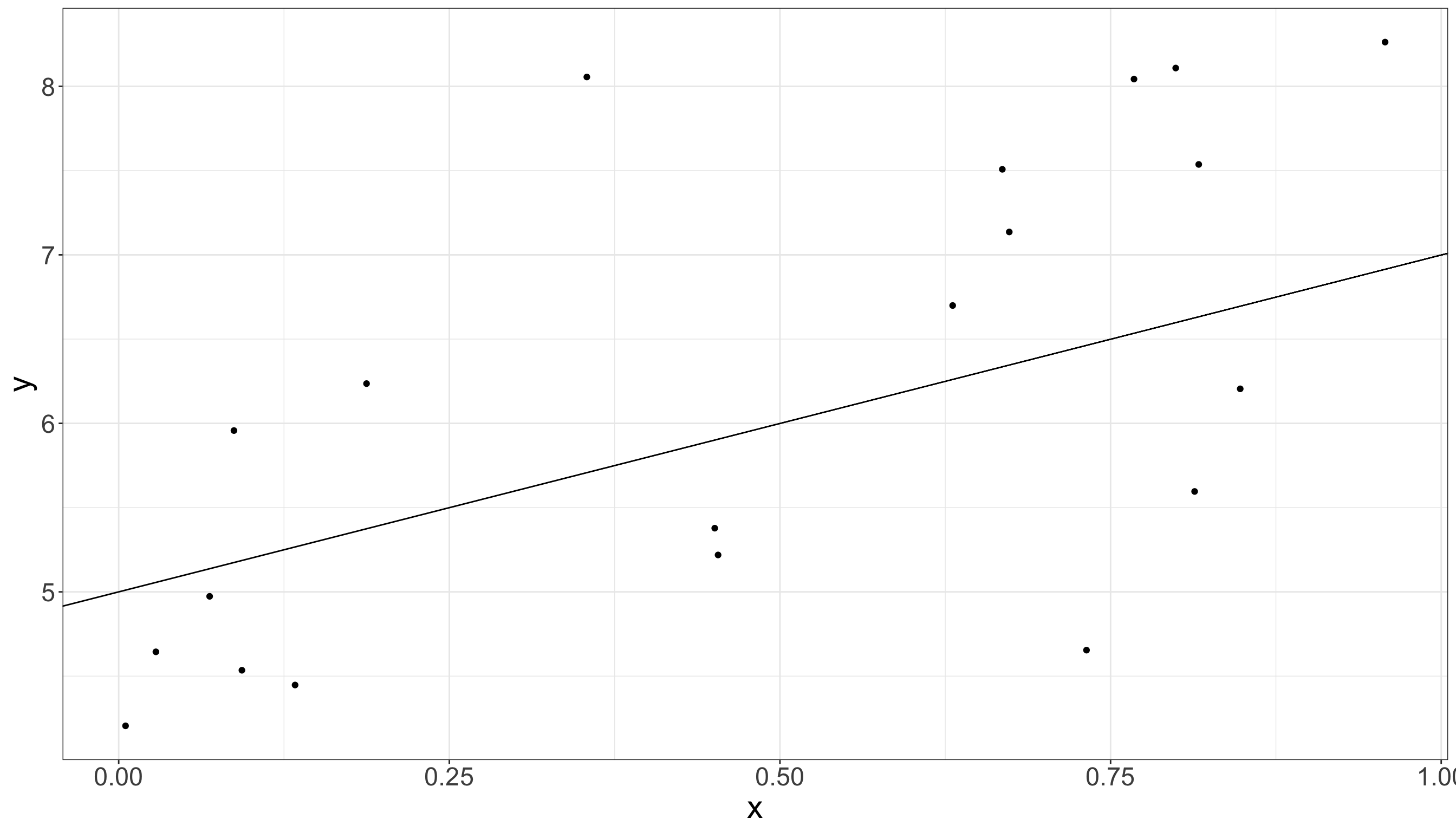
Figure 1: Scatter plot with true linear model overlaid.
Ordinary linear models are great, I love and use them all the time. However, there is a key assumption when writing that cute little “iid” in the \(\epsilon \stackrel{iid}{\sim} N(0,\sigma^2)\) that can cause us all sorts of problems.
Assuming Independence
By writing those three little letters on top of that little squiggly line, we’re making a strong assumption about how we think those data are generated. In effect, we’re saying that each \(y_i\) does not in anyway depend on any other \(y_i'\), or more formally, for any \(i\neq i'\), \(P(y_i|y_{i'}) = P(y_i)\): the probability of \(y_i\) being equal to some value is the same whether we observe \(y_{i'}\) or not!
As you can imagine, this is often not the case! In the context of the built environment especially, where we may be concerned with estimating the rate of crime, traffic, human health outcomes, economic productivity, etc., we’d often expect to find that the measurements in one area are very similar to the rates in an adjacent area. This idea is so well established, that in the field of geography it has been given high status as a “law.”
“everything is related to everything else, but near things are more related than distant things.” - Waldo Tobler’s First Law of Geography
Still, even after all this exposition, you may find yourself asking a particularly titular question.

Spatial Models
Spatial models, as well as many other classes of models, remove the independence assumption by assuming some structural form of dependence between observations. Accounting for this is not only crucial to conducting valid inference — our ability to credibly identify the effect of some exposure or intervention of interest — it also helps us to better predict measures in areas where we might not otherwise be able to collect data. The manner in which this dependence or correlation between observations is formed depends on both the system under study as well as the data collected.
Spatial Surfaces
Air pollution, tree cover and carbon dioxide levels. Each of these represent a kind of continuous surface across space that one may be interested in modeling but would likely need to account for spatial dependency in so doing. A common method for modeling this class of data is the Gaussian Process (GP), used as a spatial random effect, analogous to a typical random effect, as described in (Fitzmaurice et al. 2008), but now explicitly modeling the spatial dependence, or covariance between two observations, \(\Sigma_{i,i'}\),1 through a covariance function \(\Sigma_{i,i'} = \kappa(\mathbf{s}_{i},\mathbf{s}_{i'})\), where \(\mathbf{s}_{i}, \mathbf{s}_{i'}\) represent two different spatial locations:
\[ y_i = \alpha + \beta x_i + b_i + \epsilon_i \\ \mathbf{b} \sim MVN_n(\mathbf{0},\Sigma) \\ \epsilon_i \sim N(0,\sigma^2). \]
For example, suppose we look at the EPA’s ozone measurements over Allegheny county for the month of August, 2021, shown in Figure 2.
Figure 2: Visualization of average ozone air quality data across Pittsburgh monitors during August 2021. Data taken from the EPA.
Even though we only observe specific points, we understand that the ozone levels could be continuously observed across the entire county. Fitting a GP model allows us to estimate that underlying spatial dependence and use the few points we observed to interpolate across the wider space: Two \(b_i\), \(b_{i'}\) terms will be more similar the smaller the distance is between the two points’ spatial locations.
Looking at Figure 3, you can see this point illustrated. While we only had a small number of points available, we can now see the estimated surface across all the neighborhoods of Pittsburgh.
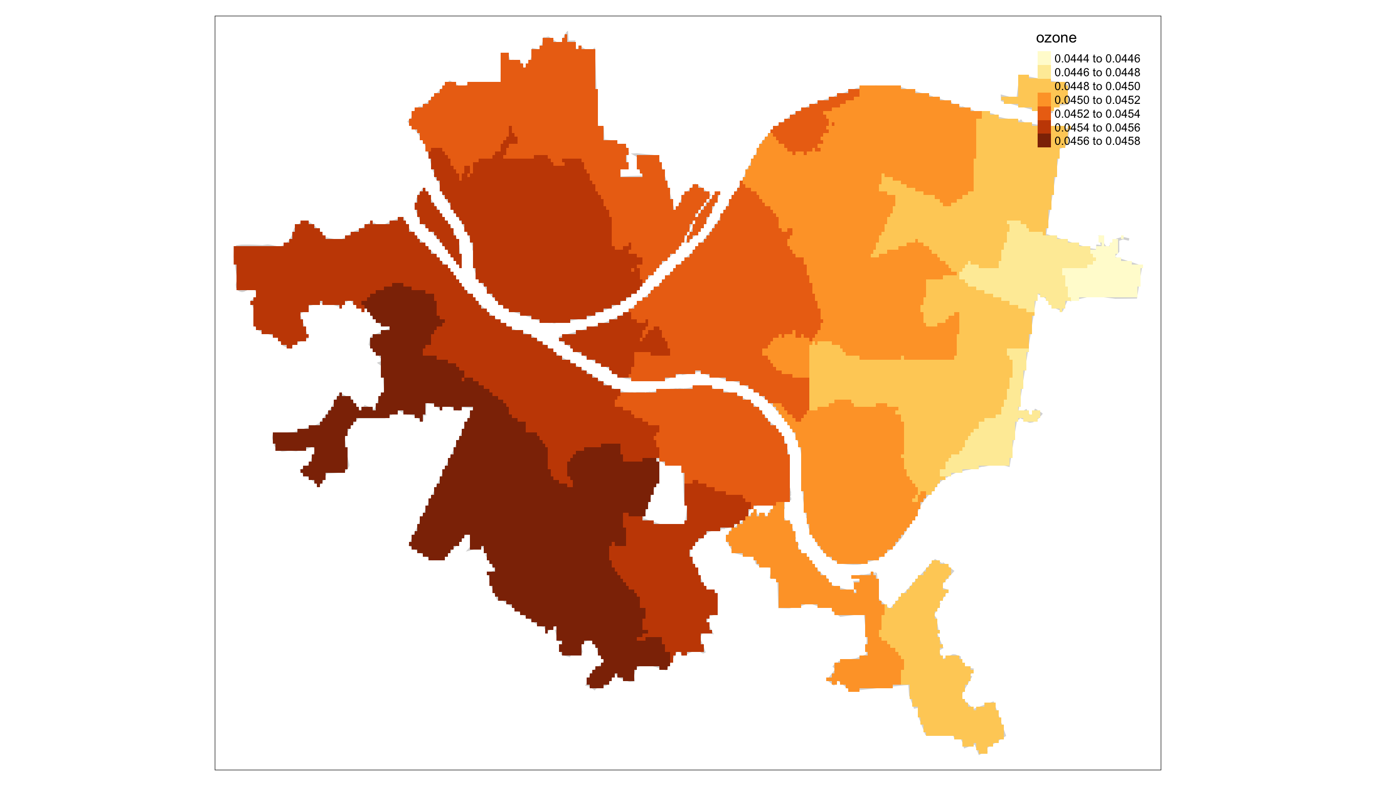
Figure 3: Estimated Ozone Surface across PGH using Neighborhood Centroids as prediction points for each Neighborhood’s surface.
Areal Spatial Networks
In contrast to points that we know are surfaces, we can also observe measures at an areal level: census tracts, neighborhoods, city streets, etc. where the spatial correlation isn’t understood in terms of the distance between two points, but rather the adjacency of the two observed units in space.
For example, in Figure 4, we can see the median income across the different census tracts of Allegheny county. Each tract is adjacent to several others. In modeling the median income across space, we might expect those tracts adjacent to one another to have similar median incomes.
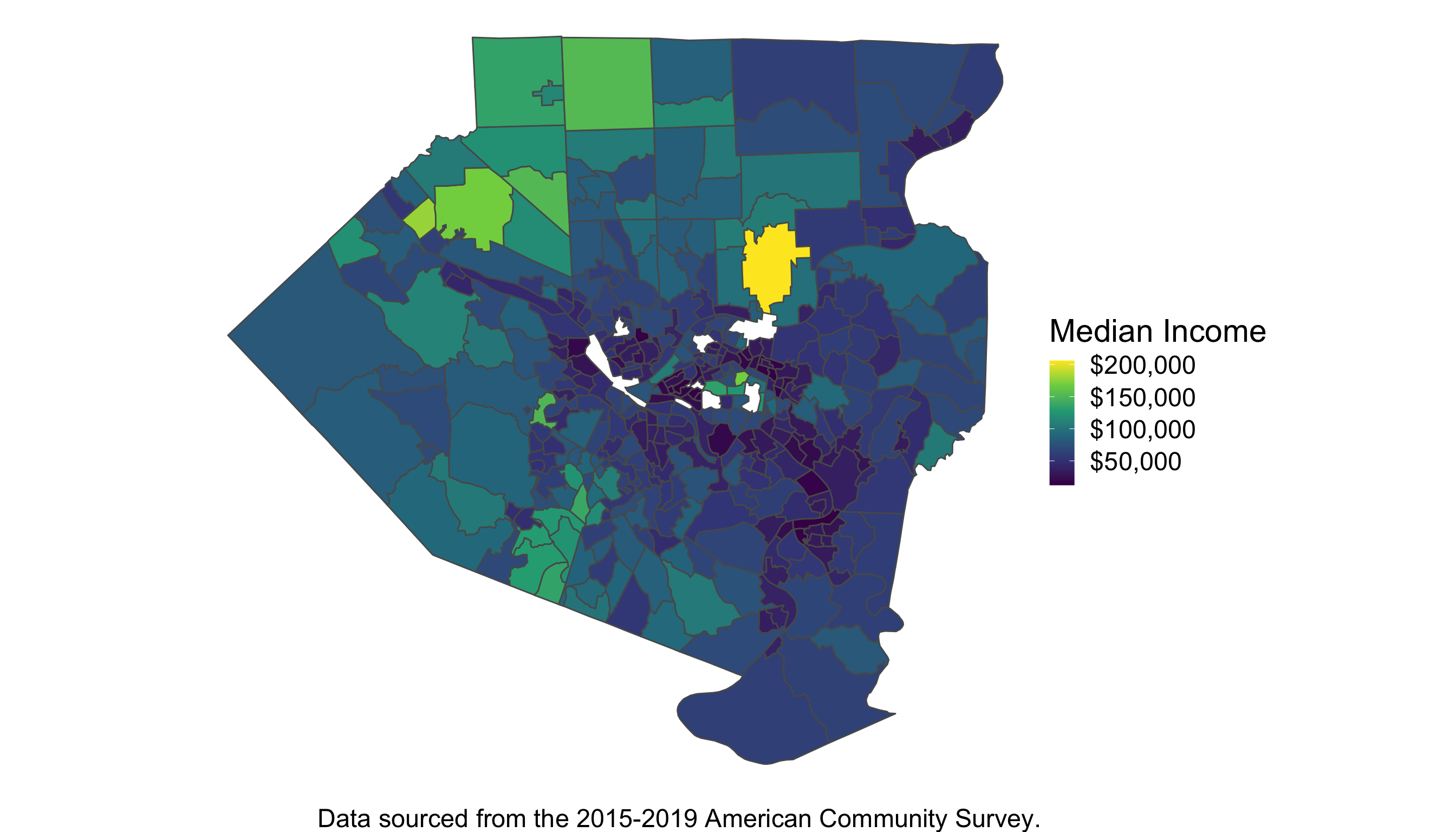
Figure 4: Distribution of Median Income Across Allegheny County, PA Census Tracts.
One way we can try to capture this notion of network dependency is through the Conditional Autoregressive, or CAR model shown below:
\[ y_i = \alpha + \beta x_i + b_i + \epsilon_i \\ \mathbf{b} \sim MVN_n(\mathbf{0},\Sigma) \\ \Sigma = \tau D(I-\alpha \mathbf{A}). \]Where before the correlation between two points, \(\Sigma_{i,i'}\), was a function of the distance between those points, now it is a function of the adjacency matrix \(\mathbf{A}\) which has a 1 in row \(i\) and column \(i\)’ if the \(i\)th and \(i\)’th observation are adjacent and 0 otherwise.
Similar to how we could use the \(\kappa(\cdot,\cdot)\) function in the GP to learn the correlation of observations across space, the CAR model uses the adjacency matrix and associated parameters to learn the how measures may be correlated across the spatial network of observations.
Spatial Point Processes
Last, but certainly not least, we have spatial point processes. While you may be thinking, “Wait, didn’t we already talk about points?” you’d be half right. In discussing spatial surfaces we observe points, but we model the points as a continuous surface. Spatial Point processes are not only observed as points, they are also modeled as points.
Consider the locations of your favorite nearby fast food restaurants (FFRs). These can be plotted as points, as in Figure 5, and modeled as realizations from a point process.
Figure 5: Fast Food Restaurants (FFRs) and Schools across Los Angeles.
Questions surrounding point processes may once again involve examining how the points are spatially correlated across space, identifying which points in space are most likely to produce the points of interest, or even simply using the points as data to condition on in some other model of interest.
For example, in the FFR example above, we may be interested in how the FFRs are distributed across space from the schools. In this setting one could model the set of distances, \(\{d\}_{i=1}^{n}\), of the FFRs from the schools as arising from an Inhomogeneous Poisson Process (IPP), estimating the spatial intensity function, \(\Lambda(d)\), of how likely a FFR is to be located at distance \(d\) from a school.
\[ \{d\}_{i=1}^{n}|\Lambda(d) \sim \text{IPP}(\Lambda(d)) \]Conclusion
This has been a whirlwind tour that I hope has given a taste of what spatial models look like and how they can be used. These models will likely come up again and again throughout the course of this blog, as so many objects in the built environment are studied across space, so they are worth understanding early-on conceptually before they start to pop up in a “real-world” setting.
Acknowledgements
Thanks to Kevin Putschko and Robert Svoboda for reading and offering comments on this article.
Updates
I added a footnote on 10/26/21 to clarify notation for the spatial process model.
Note here that I am slightly abusing notation. Since we said that we are modeling \(y_i\) as a function of space, we might indicate this by denoting the the covariance as \(\Sigma(\mathbf{s}_i,\mathbf{s}_i)\), outcome as \(y(s_i)\) and other spatially indexed variables equivalently. I have omitted these details for the sake of exposition so that the similarities between the different models may be more easily understood.↩︎