A First Foray into Urban Economics
Digging more deeply into the subject of urban economics, as I mentioned in my most recent book review of “Order Without Design”, has been no small affair. The subject covers a wide array of topics that are each of interest in their own right. The list includes “agglomeration economics”, transport economics and more. For my first series of posts within this subject though, I wanted to learn more about housing and housing markets.
My reasons for this are many:
I’ve put away money for several years now with the idea of it being used as a down payment and have often wondered at how houses have gotten so expensive.
Related to the first point, this topic is increasingly relevant:
- It featured prominently in the 2024 US Presidential Campaign.
- It continues to dominate city council legislation.
- Advocacy groups have formed around the issue, pushing for more or less supply.
Finally, I think there are some very interesting cultural and moral questions that surround housing. Both in terms of how it represents a fundamental need of all humans (shelter) as well as an aspiration — the American dream is synonymous with owning a single family house.
I’ll leave these last questions for the end of the series, however. To start, I’ll draw from a number of sources to form the foundation of our technical understanding of housing markets. The first, (O’sullivan 1996), will be a rudimentary theoretical introduction to the topic, drawing on a basic understanding of Supply and Demand. If you’re not familiar with these topics, I’d suggest reviewing them.
In a subsequent post(s), I plan to dig into more empirical work in the field, looking at two papers published by Ed Glaeser and Joseph Gyourko:
- “The Economic Implications of Housing Supply” (Glaeser and Gyourko 2018)
- “America’s Housing Supply Problem: The Closing of the Suburban Frontier?” (Glaeser and Gyourko 2025).
Each of these offer an opportunity to look at both the historical state of the U.S.’ housing market as well as how the market operates in the present day.
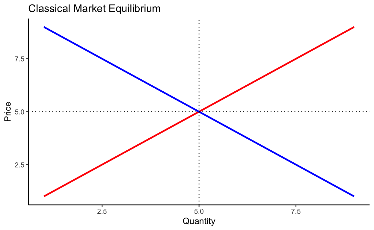
Figure 1: The ol’ Supply and Demand Curve
An Introduction to Housing Market Theory
O’Sullivan starts his chapter on Housing by noting that housing is a durable good. This means that, in contrast to an apple bought at the supermarket, a house doesn’t “go bad” after its been purchased and used by a particular consumer but can be resold later, especially if it has been maintained well. Secondly, the housing market is heterogeneous; there are different types of houses in terms of age, size, layout, etc. that can be purchased. O’Sullivan describes a “High Quality” housing market and a “Low Quality” housing market, as a simple example of how one might understand the heterogeneity in the market as well as how the two markets can interact with one another.
All of this results in what Sullivan argues is a “Filtering Model” for the housing market. Whereas in our apple example there is no interaction between the supply of a given product at a previous point in time and the present, housing supply has an explicit dependence on previous instances of supply. Sullivan formulates the model like this:
\[ H_t = H_{t-1} \times (1-f) + \text{new}, \]
where \(H_t\) represents the quantity of housing supplied at an arbitrary time point \(t\), dependent on the quantity at a previous time point \(t-1\) multiplied by some filtration rate \((1-f) \in (0,1)\), plus the addition of newly constructed housing, “new”.
The “filtration” refers to the idea previously mentioned, that high quality housing will filter down to become “low quality”, if not properly maintained. A similar expression for the dependence in low quality housing across time can be formulated as follows:
\[ L_t = L_{t-1} \times (1 - r) + H_{t-1} \times f, \]
where \(r\) is the retirement rate, of all low quality houses leaving the housing market permanently, and \(L_{t-1} \times (1-r)\) all houses that remain consequently. Adding this latter term to the houses that filtered down from the high quality market produces the total quantity of low quality houses. A natural question follows from this model - “what determines the filtering rate?”
Filtering Rate and Maintenace Costs
Intuitively, the main force is the maintenance cost. In other words, how much does it cost to keep a house in the high quality market – where the selling price will be higher – as opposed to letting it slip into the low quality market where the selling price is lower. As with all things economic, there’s an equilibrium point that defines the trade-off point, illustrated conceptually in the plot below.
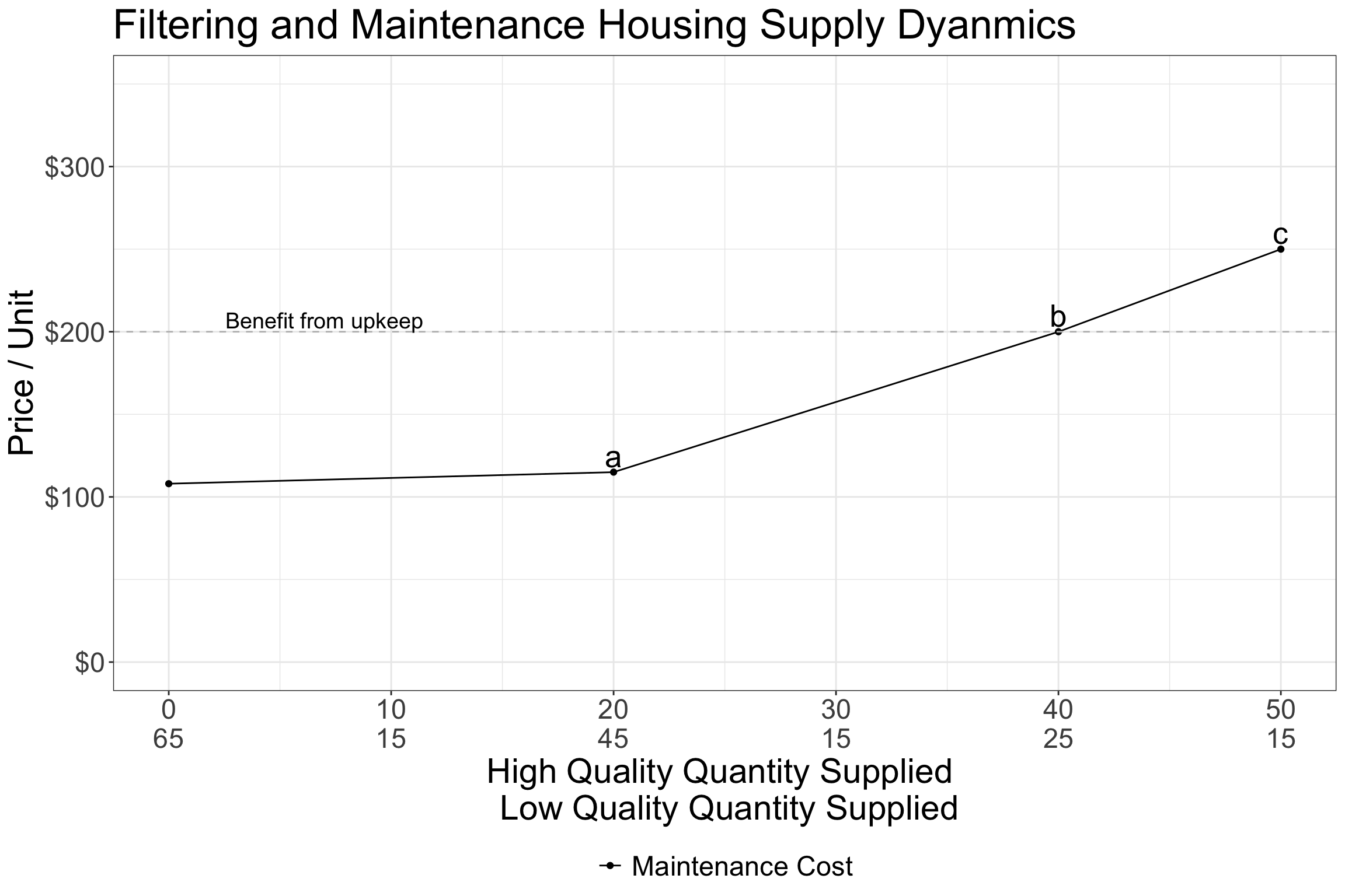
Figure 2: Maintenance and Filtering
The horizontal line in Figure 2 shows the difference between the current equilibrium (market-rate) high quality house price and low quality house price. Or, in other words, the benefit from keeping one’s house in the high quality market. If we suppose that there are a total of 65 houses in the market total, all starting as high quality, households will decide whether or not to invest in their house to keep it in the high market according to whether or not it is worth the investment. The following three cases are highlighted.
Point a: The maintenance cost is only ~$100, but if the home owner were to let their house slip into the low-quality market, they would receive less than what it would cost to upkeep it. So the equilibrium does not exist here.
Point b: The exact number of households considering letting their houses filter to the low quality market will get an equivalent benefit as those performing the necessary upkeep from the required maintenance. This is the equilibrium point.
Point c: The maintenance cost is higher than the benefit, so more homeowners will move their houses out of the high quality market, and let them filter to the low quality market.
The exact number of houses moving back and forth are determined by the market selling prices, but here the key principle is that the higher the maintenance cost – the more it costs to keep a house in the high quality market – the higher the selling price needs to be to justify that maintenance.
Filtering Rate and Market Supply Dynamics
Next, we consider how these filtering supply dynamics relate to prices in each market. Consider the plots below which use fictitious data to illustrate these concepts further.
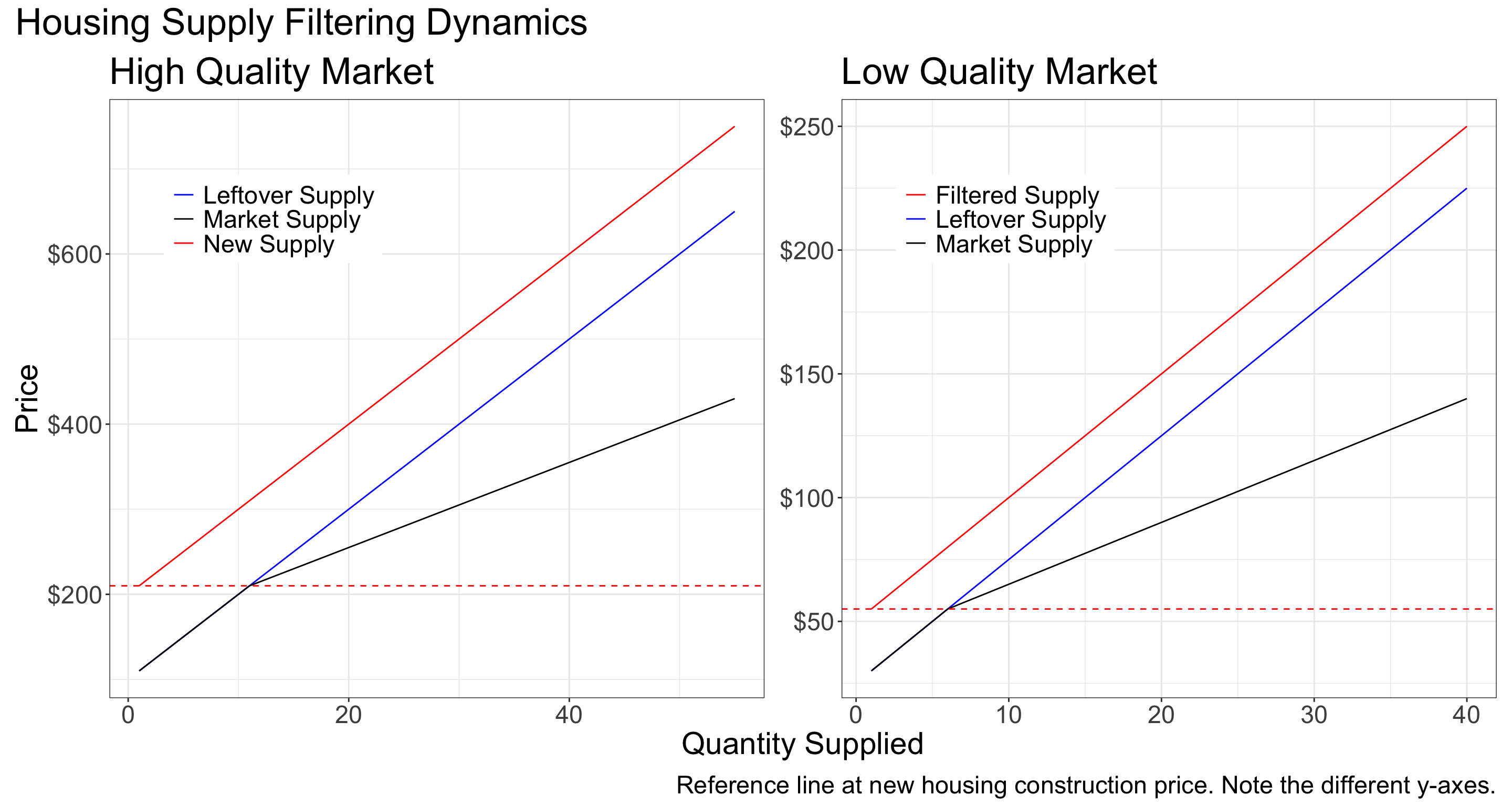
Figure 3: Supply Dyanmics in High and Low Quality Markets
Figure 3 shows the interplay between the high quality and low quality markets. In the left panel, we have new houses supplied at a price of $200 and up, with the “left over” supply starting at a lower value. It isn’t until the quantity supplied reaches a point where the price in the left over market is higher than that of the initial, or minimum, supply price for the new construction that we see a kink in the supply chain. This kink , marked by the reference line, is the market supply. The lowest of all three supply curves in price, results from a combination in quantity from each supply curve - leftover and new construction - at all subsequent prices higher than that initial entry price.
A similar mechanism is at play in the right panel. The role that new construction plays in the “High Quality Market” is played by the houses that filtered down in the “Low Quality Market”. Similar to before, the minimum price at which a filtered house enters the market is the same price at which the market will start to incorporate a greater quantity of housing from both filtered and leftover housing.
To summarize, the key principles at play in the housing market dynamics are as follows:
Housing is durable - Houses that were bought last year, could be resold this year.
Houses are heterogeneous - Houses serve different types of needs and will move from one market to another. The way in which they move is motivated by the cost of maintenance to keep them in one market, and the benefit obtained from selling them in one market vs. another.
Both of these dynamics combine — in addition to the classic economic principles of supply, demand, substitution, etc. — to form the housing market consumers and sellers participate in.
To finish off this post, let’s look at what happens when a theoretical restriction is applied to the market and the resulting changes that ensue.
An Application of the Filtering Model: Permit Restrictions
Suppose we have our same model as before but now the government has, in some way, limited the number of new houses that can enter the market. The simplest way that this can occur is through permitting. In most municipalities house builders have to obtain a permit in order to build a house. If the municipality limited the number of permits that were distributed in a given time frame, what impact would that have on the housing market?
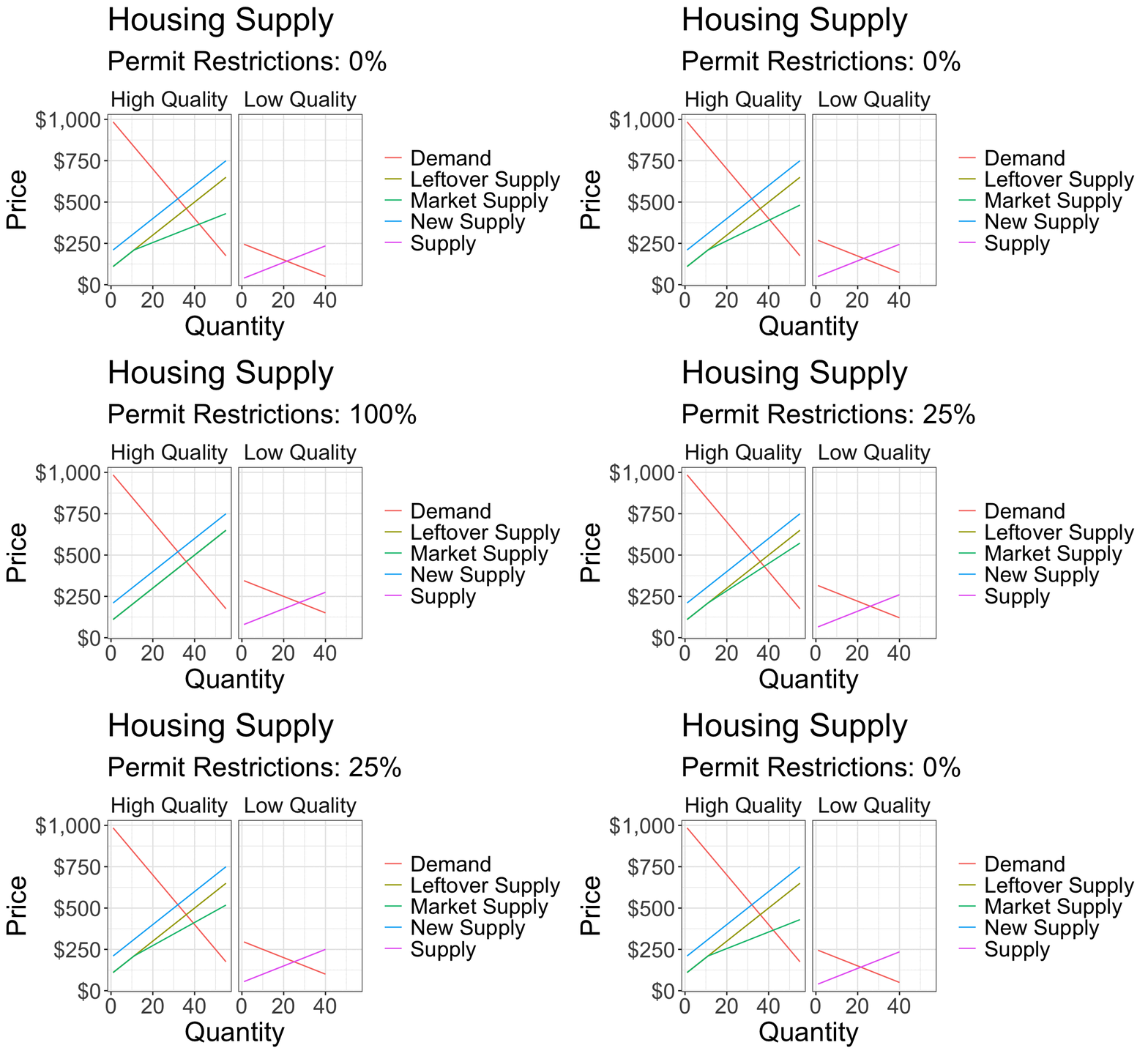
A simple, extreme case, in our permitting example would be if the government did not issue any permits for new construction. In this setting we’d see the market supply of houses restricted to the “Left Over Supply” curve. For a less restrictive case, the supply curve would move along the demand curve, in between the original market supply curve and the Left Over curve. These changes also ripple through to the Low Quality housing market via the filtering mechanism; since there are fewer houses being built, fewer houses will filter down into the low quality market. This will result in a shift in the overall supply in the low quality market upward. At the same time, O’Sullivan argues that demand will increase, as consumers will move into the low quality market since they can’t afford the higher prices in the more restricted high quality market.
All of these changes happen dynamically — the animation below shows how the market price will respond according to the permit restrictions on new construction.
While the example of permitting restrictions offers a straightforward way to understand how the market would respond to restrictions in the supply of new house construction, a similar effect would be observed under any restrictions imposed on new housing construction. In subsequent posts, we’ll examine other barriers to housing construction that arise in the US housing market and look at the evidence economists have put forward to show that, empirically, the result predicted by the theoretical models outlined above are also be observed in practice - or not!
Acknowledgements
Thanks to Paul Haluszczak for reading and offering comments on this post.