Cleanup vs. Crime: Causal Inference

What kinds of causal claims are justified from an empirical analysis?

After we’ve calculated our buffer counts and fit our fancy mixed effects regression model what kind of claims can we make about the results?

In the paper we’ve been studying, the author’s estimate a decrease in the number of crimes around vacant lots randomly assigned the greening or mowing interventions, stating in their abstract:

Conclusion: Remediating vacant land with inexpensive, scalable methods, including greening or minimal mowing and trash cleanup, significantly reduced shootings that result in serious injury or death.

Public Health Implications: Cities should experiment with place-based interventions to develop effective firearm violence–reduction strategies.

Both these and other claims the authors might make require varying level of assumptions in order to be valid. In this post, we’ll walk through these claims step-by-step, identifying the tools the author’s did or did not use to try to fulfill each assumption.

Descriptive Statistics vs. Causal Inference

Let’s start with the easiest, most defensible claim the authors can make after finishing their analysis. I’ll limit these statements to just the greening intervention since that had the more robust results across the models.

“The greening intervention was associated with a decrease in crimes in the area proximal to the vacant lots in our sample.”

There are two keywords that I’ve bolded in the above quote. The first — associated — is important because it implies that there is not necessarily a causal relationship between the greening intervention nearby crime. The second — sample — implies that the association may be limited to the sample and not generalizable to a larger population of vacant lots and shooting crimes generically found in the world at large.

These claims fall under the category of what statisticians might colloquially call “descriptive”, in that they are absolutely true in describing the sample as observed. Scientific research generally aims to establish more general truths that describe the causal relationships that determine the data we observe. In order to make the jump from describing our sample to describing the world, there are several assumptions we have to make, critical to our ability to draw a causal conclusion from our descriptive analysis.

Assumptions Assumptions

Here’s a stronger claim than the previous.

“The decrease in crime observed was caused by the greening intervention in our sample.”

In order to make the jump in claim from association, or correlation, to causation the author’s need to defend their ability to have met the identifiability assumptions for a causal effect. I’ve discussed these ideas in greater depth here and here but for now we’ll focus on (1) the author’s strategy in using their second buffer model to check for spillover effects and how this relates to the notion of of interference, as well as (2) how the author’s use of randomization should provide them with some justification for arguing that the intervention assignment is independent of other potential confounding factors.

Spillover and Interference

If a cluster of vacant lots were assigned to the greening intervention, how far would the decrease in crime associated with that intervention extend out in space? Is it possible that the effect could impinge upon another vacant lot?

Here we’re considering the spatial scale of the intervention. Just as potentially important is the temporal scale, or that time at which the intervention has its greatest impact. See (Peterson, Hirsch, and Sanchez 2021) for more on this idea.

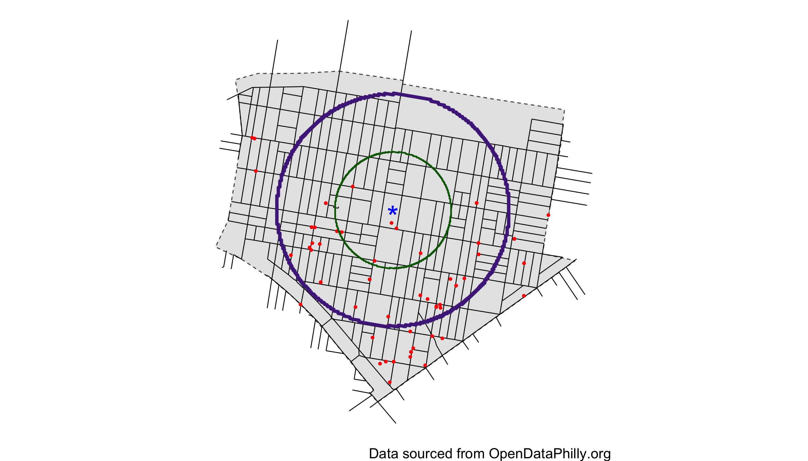
Figure 1: Illustration of buffer zones around hypothetical vacant lot. First buffer in green is used to detect proximal increase/decrease in crime, while the second is used to check for spillover effects by considering the non-overlapping area between the two circles.

Figure 1 illustrates the method the author’s used to check for “spill-over”. By looking both 300 and 600 meters around the vacant lots they sought to establish that the interventions did not simply move the shootings from closely to slightly further away, but actually did diminish the overall number of shootings. However! What the author’s failed to acknowledge and comment on in their paper, was the impact that this extended spatial impact — when one vacant lot’s effect may impinge upon another — may have upon their estimates of the intervention effect, as it demonstrates the capacity for these vacant lot interventions to interfere with one another. Recall that the author’s clustered vacant lots in order to try and limit the impact from spatial proximity, but this extended spatial effect shows the effect may go farther than previously anticipated. We’ll use this as a point of discussion in a future blog-post but for now we’ll simply consider it a question this result leaves us asking.

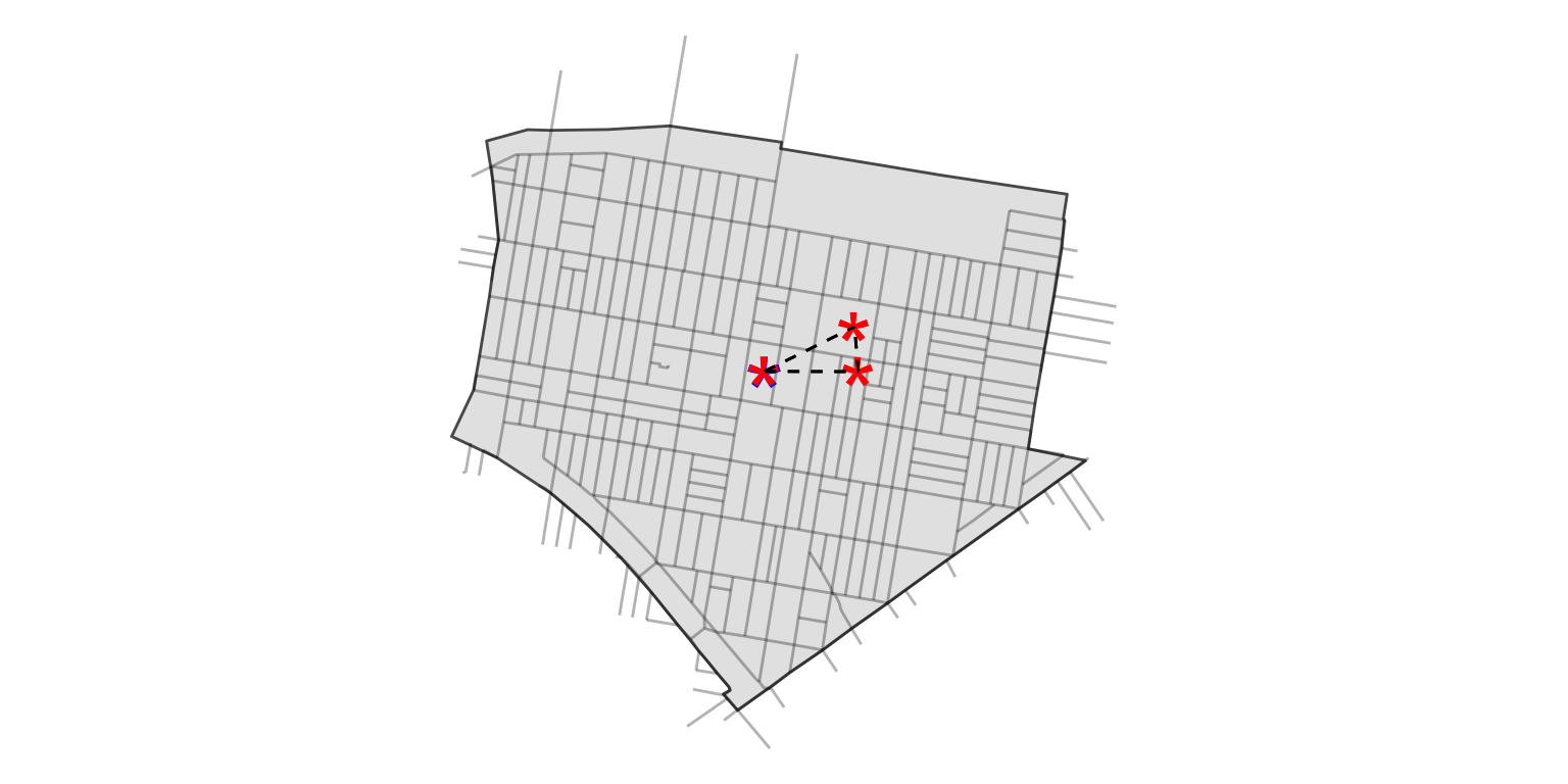
Figure 2: Visualization of hypothetical vacant lots proximal to one another whose effects may interfere with one another despite clustering.

Repeat Randomization

Another tool the author’s used was randomization: “A repeat randomization procedure ensured that the clusters were balanced on potential confounding variables including the total area and mean separating distance of the vacant lots, the resident population, and the number of Summary Reporting System Part I serious violent and property crimes, such as robbery and burglary.” (Moyer et al. 2019).

The authors use randomization to try and create exchangeability between the different intervention groups. That is that there is just as much likelihood of a crime occurring in the area proximal to a control vacant lot as it would in an area proximal to a vacant lot receiving one of the two interventions.

There are two things to note here, (i) the author’s are doing everything they can to try and ensure that these different vacant lot clusters are comparable across the different intervention groups and (ii), they seem to have trouble accomplishing this goal.

As they state in their results, “The greened lots tended to have a slightly higher average shooting rate in the baseline period (pre), which we accounted for in the regression estimates”. This imbalance¹ between the different intervention groups, reflects a difficult truth in built environment research and the larger realm encompassing the social sciences more generally: it is really hard to make things that are fundamentally different comparable for the sake of analysis. This may be why the authors chose to conduct their analysis using the difference-in-difference estimators, as this is not the strongest, or “best” contrast that a scientist typically hopes to make in establishing a causal effect.

Treatment Effects

Let’s continue with our hierarchy of claims.

“Applying greening interventions caused there to be a reduction in crime around vacant lots greater than one would observe otherwise.”

This is a very specific kind of claim that may be more familiar when considered in the context of a pharmaceutical clinical trial. If we were to randomly assign a treatment and placebo to a group of individuals who had some disease, we would be most interested in the difference of outcomes between the individuals who had the treatment and those who had the control. In statistics and causal inference this is called the Average Treatment Effect (ATE), and is the most frequent causal estimand of interest. If \(A_i=1\) indicates the \(i\)th subject, \((i=1,...n)\), in a clinical trial received the treatment and \(A_{i'}=0\) indicates the \(i'\)th subject received the placebo and we were measuring some outcome \(Y^{(t)}_i\) at time points \(t = 0, 1\), then we would define the ATE and estimated ATE as follows:

\[\begin{equation} \begin{aligned} ATE &= E[Y^{1}|A=1] - E[Y^1|A=0] \\ \hat{ATE} &= \frac{1}{n}\sum_{i=1}^{n} Y_i^1A_i - \frac{1}{n} \sum_{i=1}^{n}Y_{i}^1(1-A_i) \end{aligned} \end{equation}\]

Another causal estimand is the Average Treatment Effect on the Treated or ATET. This estimand is represented by the following expression, note the difference in the time points and treatment variables : \[ \begin{aligned} ATET &= E[Y^{1}|A=1] - E[Y^{0}|A=1].\\ \hat{ATET} &= \frac{1}{n}\sum_{i=1}^{n} Y_i^1A_i - Y_i^0A_i \end{aligned} \]

Conceptually the regression models the author’s used, discussed in the previous post, estimates this latter (ATET) entity, but in a slightly more complicated way. To make things simpler, this idea can be represented as the difference between the two points connected by the line in Figure 3 below.

Figure 3: Visualization of Average Treatment Effect (ATE) and Average Treatment Effect on the Treated(ATET) below using the crime density estimates from (Moyer et al. 2019). Solid line is above the two points involved in the ATET and the dotted line is above the two points involved in calculating the ATE.

Bringing these ideas back to the claim at hand, the author’s did not aim to justify this statement. By using a difference-in-difference estimator they estimated the ATET, which was their “take-home” result.

While this is still an interesting result, it does make a reader like me wonder why they went to the effort of randomizing interventions as they did, if they didn’t even use their control vacant lots in the contrast estimate of the intervention effect(s). My guess is that the result was not significantly different and they didn’t want this result complicating their story.

However, before we get too dramatic, it is important to realize that the authors do have some justification for focusing on the ATET as they did. As mentioned above, the pre-intervention crime measures for the three different vacant lot groups were all different, suggesting these may not have been as comparable as they should have been from randomization. Given that, it seems that one of the best and most conservative things the authors could do, would be to focus on the ATET as they did. Still, it is not the best one might hope for when looking to advance the cause of “place-based interventions” as I and the authors both hope to do.

Note that under an additional assumption, termed the parallel trend assumption, the ATET is equal to the ATE. This assumption is often made in natural experiments, where one cannot randomize a treatment and control group. However, it is not likely relevant here, as the author’s could explicitly compute the ATE.

Generalizability

“Greening vacant lots will reduce in crime in the surrounding area generally and not just in Philadelphia”

Separate from the ideas of ATE’s, ATET’s and randomization is the question of generalizability. How much can we hope that the results found here will be reproduced in other cities around the globe? This likely depends on the mechanism by which violent crimes manifest, as well as how greening or mowing vacant lots plays into this mechanism. The authors speak to this idea in part in their discussion, and we’ll discuss this idea further in the subsequent post discussing the substantive reasoning at play in this study. For now it might suffice to say that the more similar a city is to Philadelphia the more likely one would be to feel justified in expecting these results to apply and vice versa.

Recap and Conclusion

Let’s review the different claims made and how they each measured up in our analysis.

1. “The greening intervention was associated with a decrease in crimes in the area proximal to the vacant lots in our sample.”

This claim has the strongest level of evidence for it. In fact I’d say it is trivially true, barring any serious data collection or study design errors.

2. “The decrease in crime observed was caused by the greening intervention in our sample.”

This claim is in line with the author’s conclusion in their abstract and is supported mainly by the ATET estimate. However, there is still the potential for interference — despite clustering – to attenuate this estimate or reformulate how the effect manifests.

3. “Applying greening interventions caused there to be a reduction in crime around vacant lots greater than one would observe otherwise.”

The author’s can’t defend this claim. While they tried to make their intervention and control groups as comparable as possible through randomization, baseline crime measures between the groups were quite different, forcing the author’s to abandon any contrast estimate between groups and focus only on within group differences.

4. “Greening vacant lots will reduce in crime in the surrounding area generally not just in Philadelphia”

Yes and no. Cities are highly variable and not at all homogeneous. The more similar a city is to Philadelphia, the more likely the results may apply. However, this is true for every built environment or place-based intervention, and shouldn’t be held against the author’s good-faith effort here. Despite the fact that the author’s can’t completely defend this claim, I agree with the statement they make in their abstract, under “Public Health Implications”, that other cities should adapt the techniques and lessons tried here. Given The cost/benefit ratio, there certainly seems enough evidence to try something, Given the potential payoff.

Overall, in my judgement, this study is still quite strong, with only aspects of interference related to point 2. and lack of comparability related to points 3 and 4. holding them back from making all the claims that one could hope for from this work. In the next and final post of this case study, we’ll look through the mechanisms by which the decrease in crime may have occurred.

Acknowledgements

Thanks to Robert Svoboda and Paul Haluszczak for reading and offering comments on this article.

---

1. See Chapter 20 Section 4 in (Gelman, Hill, and Vehtari 2020) for more on this topic.↩︎