Causal Inference in the Built Environment

How can we know how to best change our environment?

If we change the zoning rules on a region of land from exclusively allowing single family houses to permitting mixed-use apartments and retail, will this increase the number of cars on nearby roads? If an individual moves to an apartment where they have a greater number of grocery store options to choose from, will they weigh less in 2 months than if they stayed at their current location surrounded by fast food? These are the kinds of causal questions asked by those interested in understanding the built environment.

I’ve written on this subject more broadly elsewhere, but want to return to it now in a setting where the complexities of working with built environment data can be more explicitly highlighted. Note that if you’re not familiar with causal inference concepts already you may want to read the previous post series linked and/or check out one of the numerous references I cite at the end of this post to get fully up to speed.

1. Difficulties with Randomization

There are a number of obstacles that built environment data typically involve when an investigator sets out to study causal relationships. The first is that, typically, it is impossible to randomize the exposure — e.g. grocery stores — of interest. Whereas vaccines, drugs, and even some government programs can be randomly assigned to individuals, it isn’t possible to randomly assign a park to a neighborhood or a certain kind of business to a specific storefront. These kinds of decisions are extremely expensive and will often involve a substantial amount of political decision making, rendering any attempt to introduce randomness a doomed prospect from the start. As the reader may be aware, randomization is key to ensuring that the units of analysis - individuals, streets, etc. - are comparable. That is, there is no reason to think that those who have been treated or exposed are any different from those in the control group, the unexposed.

If you want to see one interesting case where an environmental exposure is randomized … and the subsequent difficulty they had — see here. This paper will be discussed soon!

This is obviously not the case in the built environment. We observe differences in the underlying populations associated with certain built environment exposures constantly. For example, dense walkable neighborhoods tend to be much more expensive than their suburban counterparts. Wealth is correlated with education, as well as number of other factors and so one might expect a wide range of different health outcomes between those in walkable neighborhoods and their more rural counterparts that are not due to the built environment at all, but rather the wealth and/or education with which they are correlated. Adjusting for these factors in order to create as comparable a comparison as possible is crucial, if one is to trust the resulting causal estimate.

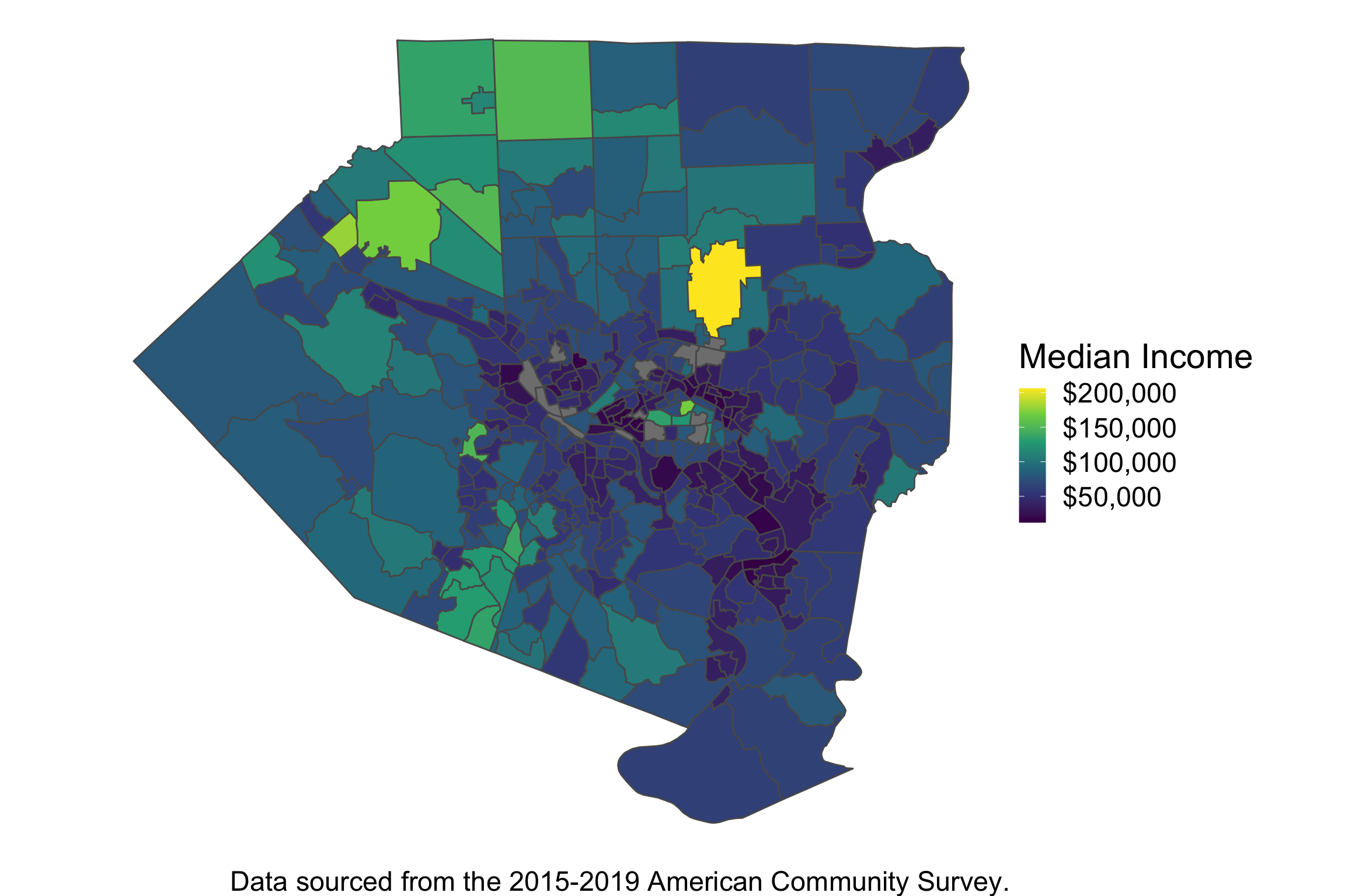
Figure 1: Distribution of Median Income Across Allegheny County, PA Census Tracts. Note the correlation in wealth across space.

2. Interference

Even if one were able to randomize exposure to some built environment feature¹ (BEF), one then has to consider the effects of interference. Interference is the name given to the phenomenon when an intervention or treatment on one entity affects the outcome of another. A violation of the commonly held Stable Unit Treatment Value Assumption or SUTVA, interference rears its heads often in the built environment.

Consider our example with upzoning. Changing the zoning on a plot of land will likely affect not only the number of cars on the street immediately in front of it but also other nearby streets. These streets traffic levels can “interfere” with one another, making a simple causal estimate more difficult to derive. Decomposing these effects across related units typically requires assumptions and/or prior understanding of the system under study. As such, interference can represent a major obstacle to making progress in this space.

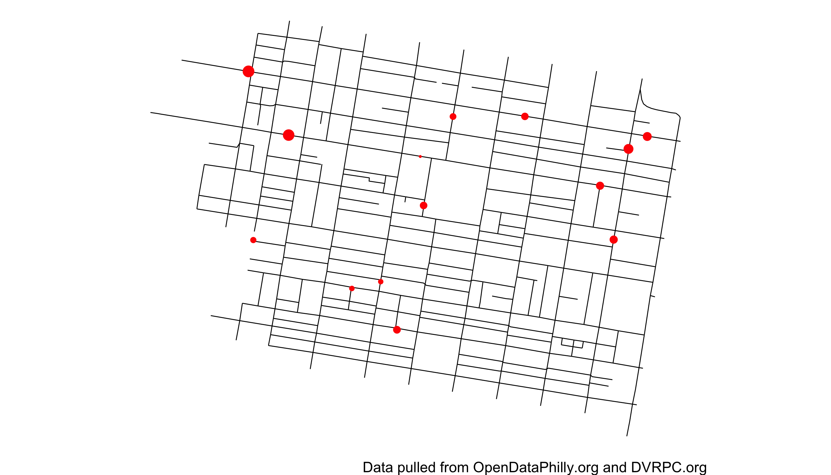
Figure 2: Observed 15 minute traffic rate on selected street blocks in Rittenhouse, Philadelphia from 2015-2020. Traffic rate is proportional to point size.

3. Homogeneity, Additivity and More

Still more problems await! In trying to understand how certain BEFs may affect human health or other aspects of the built environment, we’ll likely have to make even further assumptions. In our example with grocery stores, we’ll likely need to make some assumption that say, Kroger and Meier are equivalent grocery stores. This could be more justified than saying that the local farmer’s market could also merit the label of a “grocery store.” Assuming homogeneity in this manner greatly simplifies our modeling, and potentially increases our ability to detect an effect, but also runs us into conflicting with an assumption of consistency at the heart of causal inference.

Additivity is another such assumption that simplifies the mathematical tools required to estimate the causal estimand² of interest. However, just as with assuming homogeneity, the simplicity that additivity enables in our mathematical modeling may not be justified by our principled understanding of the causal system under study. For example, does each fast food restaurant one lives near add some appreciable weight that they wouldn’t have otherwise? Probably not - otherwise those individuals living in dense mixed-use areas like New York City and other big cities would be huge! The exposure effect is more likely to be log additive, but this can be more difficult to model mathematically.

See (Peterson, Hirsch, and Sanchez 2021) for an example of where these ideas are put into practice.

Even now, after listing all these challenges, I don’t want to leave you with the impression that we’ve covered everything. Other obstacles may still rear their head!

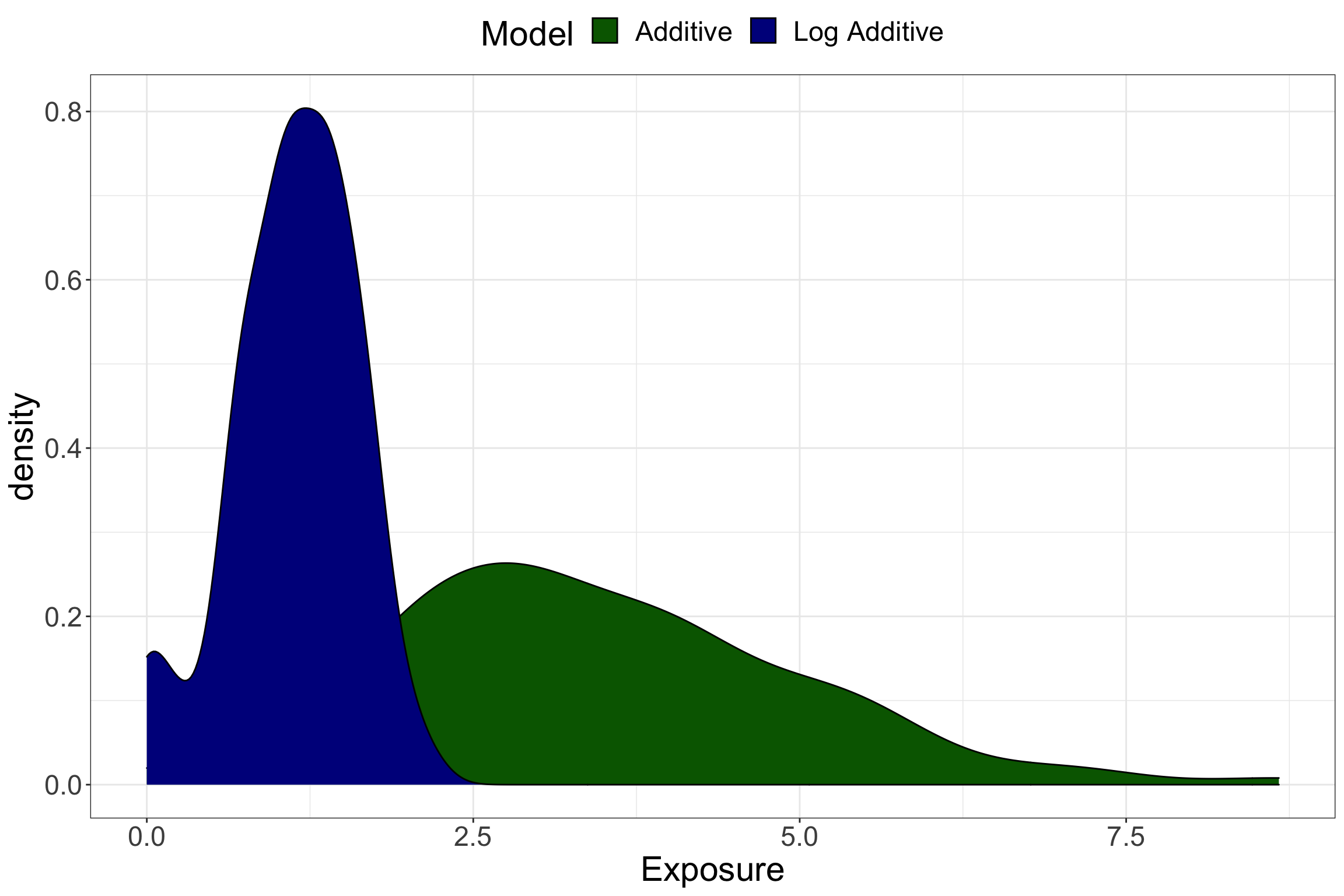
Figure 3: Differences in hypothetical exposures for additive vs. non-additive models.

Solutions

At this point, it may seem as though there is no way we can ever hope to understand the built environment amidst the many correlated and interfering forces at work. Fear not, there are still some things we can do. Though we’ll likely never have the same level of confidence in our results as we would in a randomized control trial, we can try to incorporate more information through regression, narrow our focus with difference in difference estimators, model the interference associated with interventions, and allow for heterogeneous treatment effects in our model estimates. All this and more will be discussed as a part of blog posts to come but if you’re interested in learning more of the theory behind these ideas, I’d suggest you check out the statistics references linked to on this site’s reference page and cited here (Hernán and Robins 2010; Gelman, Hill, and Vehtari 2020; Angrist and Pischke 2014; Morgan and Winship 2015).

Acknowledgements

Thanks to Robert Svoboda for reading and offering comments on this article.

---

1. Catch-all term referring to any amenity or structure in the built environment. Examples include sidewalk availability, grocery stores or tree cover.↩︎

2. an estimand is the thing one wishes to estimate.↩︎