Cleanup vs. Crime: Methods of Analysis

From KDEs to Difference-in-Differences

In the previous post we discussed this fantastic article, (Moyer et al. 2019), which studied how different cleaning “interventions” applied to vacant lots had the potential to affect the rate of nearby violent shootings. In this post we’ll look at the specific measures and statistical methods they used to analyze their data in order to test this hypothesis and break down the methods’ various advantages and disadvantages.

Methods

Data and Questions

Recall from the paper that the authors had shooting data accessed from the Philadelphia Police Department, and vacant lot data - location, size, and randomized intervention, that they amassed as part of their project. I’ve already shown, visually, what the shooting data looked like in the first post. The data structure for the vacant lot data probably looked something like what’s in Table 1.

Table 1: Hypothetical Vacant Lot Data

Lot Cluster ID	Intervention	Latitude	Longitude
1	Greening	0	0
2	Mowing	0	0
3	Greening	0	0
4	Control	0	0
5	Control	0	0

But all this begs the question, if we have lots at one location, and shootings at another, how do we relate the two to each other? The authors propose two methods, the first involving a kernel density estimate and the second involving a count of the number of shootings inside a “Buffer” Zone around the vacant lots.

Kernel Density Estimates

What’s a kernel density estimate(KDE)? Simply put, it is a fancy word for a fancy kind of average¹. The author’s created a grid of points across the polygonal space defined by Philadelphia’s borders and at each grid point took a weighted average of the number of shootings during the time period, e.g. month of interest. They chose a bandwidth of 500 meters, which essentially means that shootings within that distance were weighted more than those further away. We can’t know which kernel they used because they don’t state it explicitly, but of the many options they may have chosen the rectangular kernel, as they state many of their estimates in terms of Crimes per km\(^{2}\). The KDE,\(Y_{it}\) at an arbitrary location \(\mathbf{s}\) for a given month would then combine all \(i=1,...n\) shooting samples as follows: \[ Y_{it}(\mathbf{s}) := \frac{1}{(0.500)^2}\sum_{i=1}^{n} I(\mathbf{s}'_{it} \in U), \] where \(I(\mathbf{s}' \in U)\) is a function that returns a 1 if the location of shooting \(i\) is in the box \(U\) of coordinates defining a 500 m\(^2\) square around location \(\mathbf{s}'_{it}\) during time period \(t\) and 0 otherwise.

Again, what this amounts to conceptually is an average number of shootings at each grid point, where those shootings at closer distances are weighted more and those shootings at further distances (those more than 500 m) are weighted zero. The authors create their main figure in the paper from plotting the relative averages at each grid point across space. The lower values are assigned a light green color and the higher values are assigned a red color. See Figure 1 from their paper, below where the shootings are calculated at at yearly rate.

Figure 1: Kernel Density Estimate of shootings Figure from (Moyer et al. 2019).

As you can see, the kernel density estimate gives us this nice visualization and a decent conceptualization of the vacant lots that are most prone to having shootings nearby, but what are the disadvantages, if any?

Pros and Cons

As stated previously, the KDE has a number of advantages, including the ability to nicely visualize across continuous space, the relative “amount” of shootings at each location. However, it has a number of drawbacks too. The first, is that we don’t know if it’s a particularly good estimate. If you recall, the author’s chose a certain bandwidth of 500m, but wouldn’t 400m have been just as good? This is a well established problem in this space known as the modifiable areal unit problem (Fotheringham and Wong 1991) (MAUP), which formalizes the notion that different bandwidths or buffer choices correspond to different levels of exposure – exposure to cleaned vacant lots in this setting – and consequently different estimates of how exposure may affect the outcome.Further, while the idea of a KDE of shootings can be nicely visualized, as in Figure 1, it can be difficult to communicate verbally to stakeholders:

“Ah yes, you see when we cleaned up these vacant lots we found that the average number of shootings at the vacant lot decreased as measured by this kernel density estimate, which takes into account a weighted average of those shootings that are nearby. What do I mean by nearby and how did I choose the weights? Well the weights and proximity are defined according to this kernel and bandwidth measure we chose…”.

You get the picture. It would be much easier to say, did the average number of shootings at location “x” go down or not? However, this can be much harder to model, so the authors, understandably, went with the KDE. The outcome in their first model, \(Y_{it}\), was consequently defined as follows:

\[ Y_{it} := \text{ KDE at lot } i\text{, in study month } t. \\ \]

Buffer Counts

The second measure the author’s use to try and assign a specific number of shootings to a vacant lot is known as a “buffer count” or “buffer zone”. Put simply, the author’s looked at the center of each vacant lot, drew a circle 300 meters around that point, and counted all the shootings that fell into that circle, during a given month and assigned that value to the vacant lot as it’s count of shootings, \(Y_{it}'\). See Figure 2 for a visualization of this idea. The authors then went on to check for “spill-over” effects through the use of a second, 600m buffer around the first.

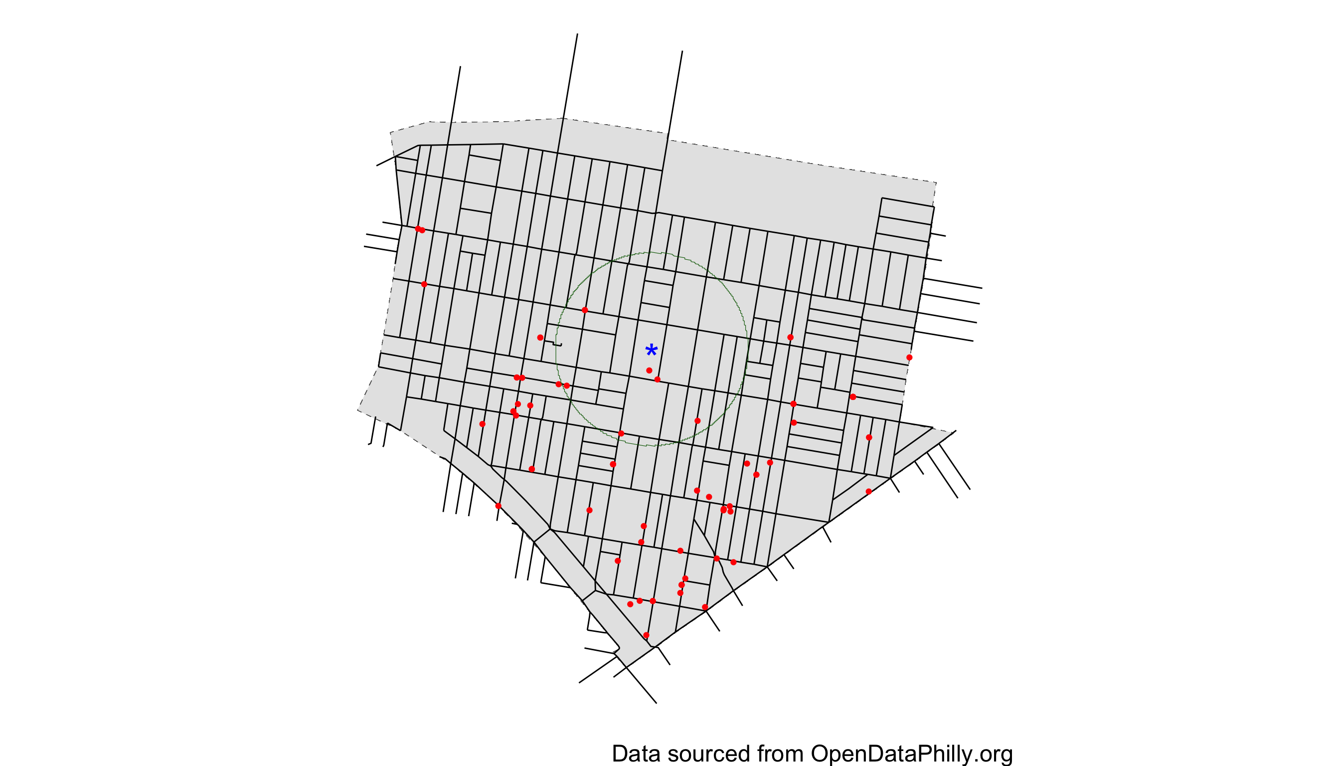
Figure 2: Visualization of Hypothetical Buffer with 300 m radius in Upper Kensington. Star represents location of hypothetical vacant lot.

Pros and Cons

The buffer count has a very appealing interpretation as it is simply the number of shootings within a certain distance of the location of interest. This is much easier to explain to stakeholders, and others who may be interested in this work, but not interested in learning about kernels and bandwidths. It can also be seen as a kind of kernel density estimate, except now we’re taking an unweighted, unnormalized average². However, similar to the kernel density estimate, it suffers from the MAUP by having to choose some ad hoc distance, 300 (or 600 for spillover) meters in this case, as the “correct” distance within which to count shootings. This remains a major drawback.

There have been developments in the statistics literature to try and address these issues that we’ll discuss in detail at another point in time. See (Baek et al. 2016),(Peterson, Hirsch, and Sanchez 2021), and (Peterson, Sanchez-Vaznaugh, and Sanchez 2021) if you’d like to learn more now.

\[ Y_{it}' = \text{# of shootings within 300m of vacant lot } i \text{ during month } t \]

Difference in Differences

Now that we have our two outcome measures constructed from the shooting data and vacant lot locations, we can turn to modeling the potential effects of the vacant lot cleanup intervention. The author’s estimate a “Difference-in-Differences”(DnD) of the expected number of shootings at the lots that receive either the “greening” or “mowing” intervention. This is a very specific estimate that we’ll elaborate on in more detail in the causal inference post, but for now it suffices to say they’re comparing the same vacant lots before and after receiving the interventions, as opposed to comparing those lots that received interventions and the control. ³ For now, let’s break down this big equation from the initial post and try to understand how they calculate the difference-in-difference estimate for the greening intervention⁴;

\[\begin{equation} \begin{aligned} Y_{it} &= \beta_0 + \beta_1 \text{Greening}_i + \beta_2\text{Mowing}_i + \beta_3\text{Post}_t + \beta_4\text{AllTreated}_i \\ &+ \beta_5 \text{Greening}_i \times \text{Post}_t + \beta_6\text{Mowing}_i \times \text{Post}_t \\ &+ \beta_7\text{Greening}_i\times \text{AllTreated}_t + \beta_8\text{Mowing}_i \times \text{AllTreated}_t \\ &+ \alpha_{m(t)} + \delta_{s(i)} + \xi_{c(i)} + \epsilon_{it}, \end{aligned} \tag{1} \end{equation}\]

This equation uses the notion of indicator functions. That is, Greening\(_i\) is either a 0 or 1 for lot \(i\). 1 indicates the lot received the greening intervention and 0 indicates it did not. Post\(_t\) is the same where a 1 indicates the measurement was recorded after the intervention was administered and vice versa.

From (1), we can see that the expected number of shootings for a greening lot prior and subsequent to the intervention is represented by \(\beta_0 + \beta_1\), and \(\beta_0 + \beta_1 + \beta_5\), respectively. If we want to know the difference then, in the expected number of shootings for the same vacant lots assigned to the greening intervention before and after the trial, we simply take the difference between these two equations which gives us \(\beta_5\). Our estimate of this quantity, \(\hat{\beta}_5\), is the estimated effect of the greening intervention. Similarly, \(\hat{\beta_6}\) is the estimated effect of the mowing intervention.

Of course, in statistics it isn’t sufficient to just calculate a point estimate, like \(\hat{\beta}_5\), and call it a day. We need to provide some measure of our uncertainty of that estimate as well, to establish whether this result provides enough evidence to be considered credible, or whether the estimated effect is just due to measurement error or random variation. An important part of estimating that uncertainty is taking into account sources of correlation in the measurements. The authors do this by way of incorporating mixed effects. See (Fitzmaurice et al. 2008) for a more general introduction on this topic, as we’ll focus only on those aspects relevant to this application in the following section.

Mixed Effects Regression

At the very end of (1) you can see four terms reproduced below for easier focus:

\[ Y_{it} = ... + \alpha_{m(t)} + \delta_{s(i)} + \xi_{c(i)} + \epsilon_{it}. \]

Each of the first three of these terms account for a different source of correlation between the different vacant lots. The sources of variation and the corresponding parameter are as follows:

1. Temporal correlation
   • vacant lots have similar numbers of shootings according to which seasonal month of the year the measurement is taken: \(\alpha_{m(t)}\)
2. Spatial correlation
   • vacant lots that are closer to each other will have more similar numbers of shootings than those that are far away : \(\delta_{s(i)}\)
3. Cluster correlation
   • vacant lots in the same cluster will have similar numbers of shootings: \(\xi_{c(i)}\)

The final term \(\epsilon_{it}\) represents measurement error that applies equally to all vacant lots, regardless of space, time, or cluster.

There is a lot that could be said about these mixed effects terms. However, it suffices to say that the author’s correctly include these terms to assure that the resulting confidence intervals they calculate for their estimates of interest, \(\hat{\beta_5}\) and \(\hat{\beta_6}\) take into account the variability within seasons, space and cluster.

Conclusion

In this post we’ve examined how the author’s use of KDEs, buffer counts, DnD estimators and mixed effects regression came together to try and provide a reliable estimate of the effects of the greening and mowing vacant lot interventions on shooting crimes. We’ve also seen some of the advantages and disadvantages each of these approaches may involve. Many of these will continue to be of importance as our attention now turns to the causal inference assumptions underlying the statistical methods and estimation procedures discussed here that, if correct, extend the results from this experiment to a more widely generalizable result.

Acknowledgements

Thanks to Robert Svoboda and Paul Haluszczak for reading and offering comments on this article.

---

1. This describes most of the work done in Statistics.↩︎

2. also called a sum↩︎

3. There may or may not be good reasons for not estimating this latter contrast but we’ll save that discussion for the causal-inference post.↩︎

4. I omit the distributional assumptions on the random
   effects and epsilon term here for space. They are all distributed Normal with mean zero and unknown variance.↩︎